Statistical Graphics and more

Today is the 100th anniversary of the Titanic disaster and it is all over in the media – ranging from movies to serious reportage. Having worked on visualization of categorical data visualization for a long time, the Titanic data became somewhat like “the mother of all demo datasets” and may be boring people by now as much as the Iris dataset does for multivariate analyses.

Nonetheless, there are two issues (which can be found in past posts on this blog), which summarize the most important facts on how the disaster was handled:

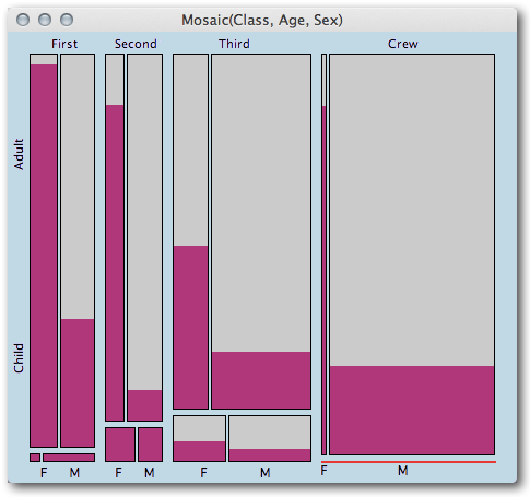
1. “Women and Children first!“

(each rectangle shows a combination of Class x Age x Sex) and
the proportion of survived passengers via highlighting)

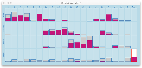
2. Travelling 1st Class makes it easier to get into a life boat …

 (Launch sequence of life boats – woman highlighted)

The shocking result of this visualization is that the first 6 boats were exclusively used for 1st class passengers (although boat No. 1 was not filled at all), and it took another 4 boats until 3rd class passengers were considered to be saved. Starting with the 15th life boat, chaos spread, and the last three boats went afloat almost empty.

Looking at the two visualizations, shows clearly what fuels the stories (not only) in the Titanic movies. 2nd class males are among those with the lowest survival rate, indicating a very heroic attitude. The boat filling strategy shows a strong social bias, which can only partly be excused by the coincidence of passengers locations and boat locations.

(Here is the data on the passengers and boats used for the visualization)

 

 

Some weeks ago I was browsing through the categories of TED Talks and was surprised to find an entry on statistics – which is regraded to be a very boring topic by most people.

The talk I chose to watch was by Nic Marks – as I tried to avoid yet another Hans Rosling talk.

Apart from Marks’ sweeping positive charisma, what struck me most, was the very relevant question, why we choose measures like GDP or NASDAQ to measure our “wellbeing” – as these KPIs mostly measure how efficient we destroy our (or others) environment or how much we increased the imbalance of wealth within our societies.

After watching the talk I ended up at the happy planet index site, and found myself flipping through their report. On page 16, I found Figure 2, which kind of blew me away.

I don’t want to get into moral preachings here, but take your time and rethink your life and attitude and try to come up with some explanation and projection of what has changed over the last 45 years – I am curious to see your comments.

Sometimes even very simple statistics make you think hard …

On the JMP blog you find a post which uses the same data source I took for my first attempt to visualize the web of the EU debt. I found it hard to really make a point with this data. Looking at the JMP post tells me I wasn’t all too bad. Let’s walk through their visualizations:

1. The Map
   Certainly necessary for someone in the US – who knows where Portugal, Spain and Austria are; or was it Australia ..?
   But seriously, scaling the very irregular shapes of the countries outline has more problems (on the perceptual side) as benefits.
2. The Heat Map
   This graph degrades the information to a binary information of being creditor or not – be it 1€ or 1,000,000,000€. The conclusion that Germany and France are in trouble because they lend to many other countries is not convincing as it only reflects their economical power.
3. The Tree Map
   As tree maps are “only” a different representation of a tree, i.e., a hierarchy, why would you visualize a matrix with it? I can’t really  follow the chain reaction of defaults which is interpreted from this tree map. Looks a bit along the lines “if all you have is a hammer, every problem looks like a nail”.

One thing that is really not well thought about the graphs are the different color schemes between the graphs.

In the end, I think someone really needs to get “the right” data and show us “the right” visualizations such that we understand what’s going on – but hurry up, Greece might be broke by then …

Looking for a map of the french Departments, I came across this map of the population density of France on Departments level which can be found on Wikipedia – and you may guess: this is this month’s “The Bad”.

At first sight there seems to be a contradiction between the apparently continuous color scale (see here for some thoughts on coropleth maps) and the map that does not seem to give any decent insight in the geographical distribution of population density. The answer is twofold.

1. The color scale is not continuous but has a break between green and blue (unless you invert the shades of blue) and blue and yellow. What we would expect – in less saturated colors – looks like this:

2. For a map showing a continuous quantity, we usually would not choose so many different saturated colors.

Let’s approach “The Good” as I still need to convince you that there might be a better version of the map. In a perfect world, coropleth maps look smooth and “continuous”. For the map of France we might want to look at the distance to the capitol Paris, as France is very centralistic. This map uses a monochromatic scale and shows “the perfect world” …

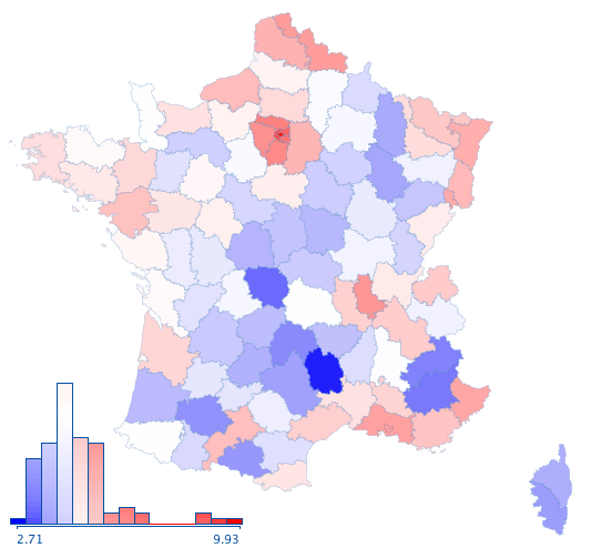
As this one is obviously too trivial, we want to look at the population density as in the above plot (2011 census data from wikipedia). Using a simple linear scale we would end up with this (useless) map, which uses a color scale that ranges from blue (small values) over white (median values) to red (large values):

Except for Paris and three other departments, all regions are unpopulated compared to the capitol. The extremely skewed distribution which is shown in the lower left, explains the dilemma.

Using the same “trick” as in the original wiki-map, i.e., cutting off all values above 150 we get a map that is easier to read, but now equalizes all information for areas above 150.

(Note, I used the histogram of log(population Density) for the legend)

The result is much better now, but there seem to be too many departments put into a single class.

From the data on the log-scale, we already see what would be most desirable, i.e., a distribution of colors, which is close to a normal distribution. Using a non-continuous transformation of the variable we display, we can map the color-shades to be normal, which ends up in the following map, which I would classify as “The Good”.

We now get a fairly good feeling of which regions are highly populated, which ones are close to the median (even with a distinction of being above or below average) and also clearly see the extremely unpopulated departments.

There is a lot more to say about the do’s and don’ts for drawing choropleth maps (which can be found here in Chapter 6). What is even more fun is to play around yourself! Here is the data (unzip and load France.txt with Mondrian) and here is the software – have fun!

(Thanks to Antony for providing the map!)

Given the trouble I got into after my post on the Japan earthquake, I probably should stay put when it comes to looking at data on hazardous events …

More seriously, as statistician (or data analyst in general) we often lack the expertise from the domain expert, who usually collected the data. Today, in a “data everywhere” world, we are in the fortunate position to easily access interesting data from various domains, but probably don’t know much about the background.

Thus I was happy to see the three posts

• Killer tornado perspective
• Tornado reports year in review
• Tornado days

on Jim’s blog. As Jim has a BS from SUNYA in Atmospheric Sciences, MS from FSU in Meteorology, and a PhD from ISU in Agricultural Meteorology, I am pretty sure he knows enough about tornados to reason beyond speculations.

You can find the data (5.5MB) here to play around yourself, which was compiled from this NOAA website. If you need a tool, you might be happy to use Mondrian.

PS: Jim agreed to write a guest post in the next few weeks, so we might learn a bit more on tornados here soon.

… which is usually Merry Christmas around here and some (still too few) Happy Chanukah.

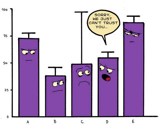
I had a good laugh when I saw Andrew’s reference to this barchart.

Maybe this is the right way to teach upper management the concept of uncertainty via confidence intervals, as the concept of mistrust is surely well known in these circles.

But to leave you with a bit of Christmas feeling, here is a great version of the ancient, latin Christmas hymn “Veni, Veni Emmanuel!”. Although I am not a particular bluegrass fan, I have to admit that this version is far closer to the original intention then what many well-meaning church choirs around will deliver.

-Enjoy!

Note: The video was recorded on Canon 5D Mark II, which gives you (given the right lenses) impressive depth of field effects – given you have the money to own a 5D MII.

Following the news and trying to understand what is going on in the “EU debt crisis” is a hard job and maybe a good visualization can help. At first sight the BBC did it. Eurozone debt web: Who owes what to whom? shows nicely how the relation between the most “interesting” debtors and creditors in the EU (spiced up with the US and Japan) is.

There is also a short explanation to each country’s situation in relation to its GDP right of the graph, but that is full of interpretations and “insights” which hardly match with the figures in the graph.

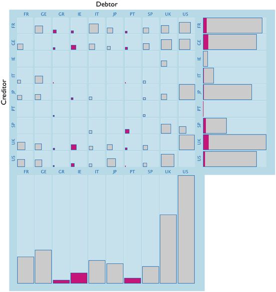
After spinning around in the debt web, I keyed in all the data, and can now create the debt matrix:

I am not sure how much more I can seen now, but I see it now all at once at least. Surprisingly (or maybe not surprisingly) the two countries which would trouble me most, are not within the Euro-Zone and don’t seem to be part of any concerns: UK and US.

One last graph which looks at the influence of the highlighted countries, which already called for help and thus have quite some potential of defaulting on their debts:

The barchart shows creditors sorted according to the share of troubled debt – though I don’t feel enlightened enough to draw any immediate conclusion form this result … I guess the data does only show a small part of what’s going on and no matter how we visualize it, we are not really getting more insight into the crisis.

Maybe it takes another post with more / better data …

It’s been a while since Georgios sent me the link to this interesting “psychogram” of iOS users vs. Android users.

In the first place I thought the really bad thing (but maybe also amusing thing) of this “analysis” is the fact that some sample has been pushed through some multivariate statistical procedure and generated some output – many opportunities for failure and no idea about significance. While this kind of “analysis” (how did you find yourself in the two worlds?) might be somewhat frightening, the real frightening thing is the site, which generated the data.

Hunch.com is a site which gives you automated recommendations about things you (apparently) like, using some “psychogram” questions and sniffing your social network neighborhood. From a statistical or machine learning point of view the task is clear: classification and prediction; from a personal point of view it might feel a bit disconcerting. Each individual, no matter how smart or dumb, is far more nuanced than the few dimensions set up in the model hunch.com might use. In the end, hunch.com does not do this out of pure altruism, they want to sell you stuff you otherwise would not have bought which makes them put us into categories we probably don’t fit into.

Statistics can be of great help in many places, but we should not actively hand over our interests to the results of some data mining algorithm.

This was not meant to be a Good & Bad, but it turned out, that the argument is most effective, when it goes beyond pure criticism and actually offers alternative – so we need a Good.

We find this nice illustration of German energy data at the GE visualization site:
This kind of visualization is quite common now and had its “initial public offering” with “The Baby Name Wizard” by Martin Wattenberg. The stacked display has some issues (which can make it to “a Bad”) and it takes a careful construction to make sure it is well readable (it actually “only” needs the right stacking order – if there is one). What struck me with above graphics was the fact, that none of the bands is actually aligned at some sort of straight base – typically the x-axis in a plot. As a consequence it is really hard to tell the story behind the data. Most frustrating, the most recent data is extremely jiggling which makes a judgement of the current trend almost impossible.

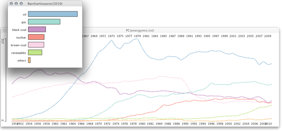
It took me a while to get the data out of the visualization, but you can actually download the whole visualization here. My first attempt to understand the data better was using simple time series which I created by “misusing” a parallel coordinate plot:
What we lose is the total, as the series are no longer stacked – though, it was quite hard to judge the total in the original visualization as well. The barchart is used as a reference and shows the most recent distribution. What can we learn from this graph:

1. Well, there was the oil crisis in 1973 – God knows what would have happened without the crisis stopping this ridicules greed for oil in the early 70s.
2. The second oil crisis in 1979 was actually having a real impact, as the decline in oil consumption lasted for four years and since then stayed on a lower level – quite contrary to the crisis in 1973.
3. Germany abandoned half of the brown coal sources shortly after the reunification.
4. Nuclear energy stalled in 2000 and is now on a (projected) decline.
5. Renewable energy sources are the only ones with a significant growth, but it still takes a long way to supersede oil and gas.
6. Coal is declining steadily.

You certainly can read off all the topics from the GE-visualization, but you probably would need to know these fact before, which is certainly the wrong way, as a visualization should generate insight and not visualize already existing knowledge.

PS: I tried to find a good stacking order, but after 30min. moving series up and down it looked like there is none.

PPS: There is a quite similar post here

Mosaic Plots are the swiss army knife of categorical data displays. Whereas bar charts are stuck in their univariate limits, mosaic plots and their variants open up the powerful visualization of multivariate categorical data.

But let’s start with an introductory example. The Titanic data is still the most convincing application of mosaic plots, though many of us saw this example over and over again – I will show other examples as well once we are done with it.

Above example starts with a simple bar chart of passengers by class at the top left, with all surviving passengers highlighted (I guess everybody is familiar with what happened to the Titanic …). The top right plot modifies the bar chart such that we can compare the highlighted proportions, i.e., the proportionality of width and height is interchanged, without changing the highlighting direction. We call this plot a spineplot.

With a spineplot, we are almost there for a 2-dim. mosaic plot, shown at the bottom of above graphic. Now we can derive the general building principle of a mosaic plot. We start with a blank rectangle and recursively split each tile according to the conditional distribution of the variable to add within that tile, e.g., we split the whole according to the distribution of class, and each class according to the second variable – in our case survived.

Leaving the survival information as highlighting, we can recursively split Class by Age and Gender and get the classical Titanic mosaic plot:

I guess it won’t take you long to find the “Women and Children first!” in the plot … (you might enjoy a video, that shows the above data visualization in action)

Now it is easy to see the fundamental difference to tree maps. Whereas in a tree map, we may split each node according to an individual criterion, the “tree” behind a mosaic plot is always fully balanced and the splits on a specific level are always according to the distribution of one fixed variable.

On the highest level, there are basically two general uses of mosaic plots.

1. Conditional Distributions
   Looking at a single response (like survival in the above example) or an interaction, conditioned on (or given a) set of variables (class x age x sex)
2. Structural properties of high-dim. categorical data
   Often we need to understand the general structure of a high-dim. categorical datasets in terms of finding empty or very small combinations, the dominating classes, or trends and patterns in the data.
   In this case we can make use of the numerous variations of mosaic plots (see, e.g., here for a Multiple Barchart), which mostly leave the strict area proportional constraint (which we need in 1.) and move to a matrix like layout (see Heike’s paper on more details, or try them out in Mondrian. See also Alex’s RMB-plots as latest contribution to this class of plots.)

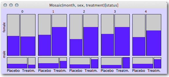
Let me give you two more examples of mosaic plots. The first is using longitudinal categorical data on respiratory diseases.

For five points in time we see the different development of the disease depending on gender and kind of treatment, with highlighted cases marking patients with a “good” status. We see the highest discrimination between the treatments for t(2) for female patients and t(3) for male patients, and a decreasing effect for t(4) for both genders.

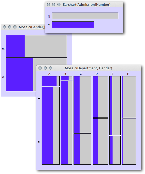
I will close with showing Simpson’s Paradox with the famous Berkeley admission data using mosaic plots:

The mosaic plot of gender with admitted students highlighted (left) shows clearly that the proportion of females is smaller than the one of males. If we split up by department (lower right plot) the share of admitted students is almost completely balanced for departments B-F and even higher for females in department A.

I leave it to the reader to find a neat verbal explanation of what is going one here (as this post is already way too long …), but so much can be said: it has to do with the proportion of females and males within the different departments.

Mac OS X Lion is now the 7th incarnation of Apple’s new operating system. Each of the version upgrades had minor additions to the graphical user interface (GUI). None of the increments did really have a big impact on how we used the OS – at least for me, things like Exposé, Spaces or the Dashboard were functions I once in a while used, but they didn’t really add to my productivity.

With Mission Control, we now have all things in one place, and it is only the next swipe away to reach the desired functionality. I think this is a good example, that often we only lack the last missing link to get to the point where the UI functions fall into place – all of the single functions where released in previous OS releases before, but only now it is completely natural to use them all – and not just once in a while.

There is certainly the “one more thing” regarding UI changes in Lion: Natural Scrolling. Just search for the comments you find on the web – they reach from “Apple’s ‘natural scrolling’ feels horribly unnatural. Here’s why.” to “Wow, Everyone’s Complaining About “Natural Scrolling” In OS X Lion“. Well to be honest, it took me a few days to adopt as well, but once you are “over it”, it just works fine (even switching back and forth between the scroll wheel on my Win PC at work and my Mac at home). It is amazing how conservative people are regarding the way they use their computer – even if it is wrong. If we did it wrong for ten years, it has to stay that way … And there is no doubt about the fact, that there is really no physical metaphor behind the direction we used the scroll wheel so far – someone just programmed it this way and we used it.

Removing the scroll bars seems to be a comparatively small interference to the user’s expectation – still having enough potential to stir users up.

To sum up, with Lion we see how little progress we made with UI improvements in the last decades – but if we really leap forward, we feel the resistive force in the user base …

This time it is easy to make a point; not because of my improvement advise being so well thought and fine tuned – no, just because “The Bad” is so convincingly bad. You find it here at slideshare, called “The Razorfish Social Influence Marketing Report”. Figure 1 on page 10 looks like this:

I would call it the most fluffy pie chart I have ever seen (and when I say fluffy, I mean fluffy – ask Agnes). We have been talking about 3-d effects, projection problems, wild use of colors or transparency misuse … but this one is really to the top as almost every thing is wrong about this chart. It deserves a seat in the hall of shame of pie charts!

My “good” is more Tufty style as it does not show axes nor annotated values, but only proportional areas and class labels:

Enjoy! (Thanks to Marco for this great example)