Statistical Graphics and more

As the FC Bayern München already won the German Soccer league many weeks ago (and consequently dropped out of the remaining contests), no one was really interested in the Bundesliga any longer – no one?

Being boring at one end of the table does not mean that the other end is boring as well. And quite opposite to the top, the bottom of the table was extremely thrilling, with 6 teams that potentially could relegate before the last match day. Even more excitingly, all 6 teams were only spread over 4 games, meaning 4 of the teams were facing a direct opponent in the fight for staying in the Bundesliga.

Enough said, within the 90+4 Minutes of match time, we saw 11 goals and 6 of these goals affected the table ranking, i.e. who was to relegate or not:

What do we learn from this visualization?

1. Paderborn, starting the last match day as last and found itself at the very same place, is to relegate. The 32 minutes of hope from 0:04 to 0:36 did fade with Stuttgarts equalizer.
2. HSV is one of the two rollercoaster teams, with a spread of 4 and 4 rank changes. Winning their game qualifies them to play against KSC of the 2nd Bundesliga, to see who is to play Bundesliga next season, as they climbed from 17th to 16th.
3. The second rollercoaster team is the VfB, with a spread of 4 and even 5 rank changes. Spending most of the last match day (exactly 55 minutes) on a direct relegation rank, winning against Paderborn pushed them up to rank 14.
4. Hannover did not take any chance and won against Hertha, climbing from 15 to 13
5. Freiburg is the looser of the day. Starting as 14th, they found themselves 3 ranks down on 17th, directly relegating to 2nd Bundesliga.
6. Hertha had only a very small chance to actually being endangered to relegate. Nonetheless, they slipped 2 ranks but as 15th, they are to stay in the Bundesliga.

Yes, it’s been a while since the last post, but hey – isn’t it a good sign that I presumably do not stumble over too bad graphics every day (or I just might not have the time to write about it …)

This example comes from SAS’s online manual on their Visual Analytics tool. And here it is:

“The Bad” is even supported by explanatory text:

“This example uses a butterfly chart to show the actual sales compared to the predicted sales for a line of retail products. The butterfly chart is useful for comparing two unique values. In this chart, the two values are arranged on each side of the Y axis.“

I am sure that my friends at SAS know better, so I won’t start bashing here, and I will also not start to refine the plot to perfection, as the problem seems to be too obvious:

Why comparing continuous quantities not side by side on the same scale, but put them on separate, opposite scales – especially when we look at quite small differences?

Maybe the programmers of SAS VA or the writers of this online help are too young, so they might have missed Bill Cleveland’s “The Elements of Graphing Data” from 1985, but they could have stumbled over this 1985 paper (available on todays internet). This paper is an essence of what the book talks about in all of Chapter 4 “Graphical Perception”, which has not changed the last 30 years (which can not be said about Figure 3.84 on page 216 ;-).

So here is Cleveland’s advice on the precision of perception tasks:

And here is the same data on a comparable scale – I hardly dare to call it “The Good”:

If someone supplies the ggplot “solution”, please feel free to comment and I will add it to the plot.

2 years ago, I did post the data on the CO₂ and global temperature relationship. The conclusion was: at least in the last 10 years, CO₂ concentration kept rising, but the global temperature didn’t.

Now, as the last year was the warmest year ever measured, it is time to look at the data again – having two more years of data.

Let’s first look at the scatterplot of temperature vs. CO₂ concentration, with the last 10 years highlighted:

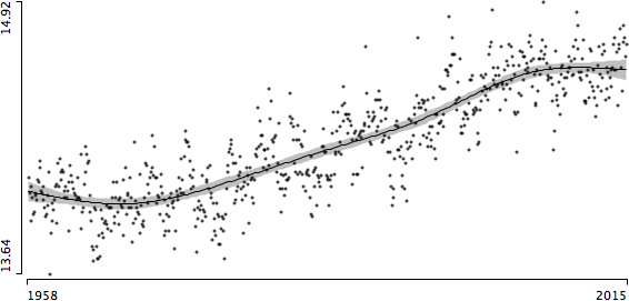
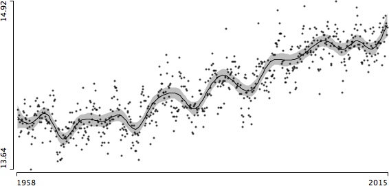
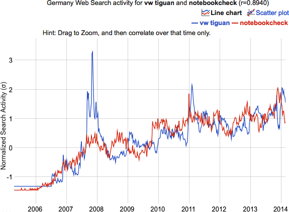
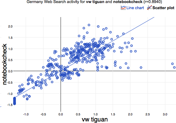
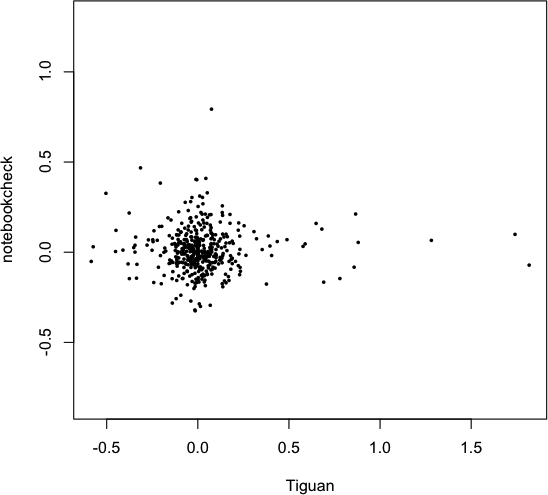
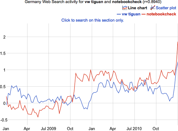
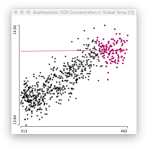
Again, there is no (linear) relationship whatsoever. Certainly CO₂ is a greenhouse gas, and we all know how a greenhouse works.

Looking at the temperature development, we can’t ignore that 2014 was the warmest year ever recorded. Nonetheless, when we use a smoother with a wider span (smoothing spline with 6 degrees of freedom), which picks up the almost linear trend nicely, the temperature rise looks like it has stalled roughly 10 years ago:

Using a far more flexible smoother (25 degrees of freedom) we get a different result, indicating a dramatic rise in temperature in the last year:

As we all know, the volatility of a trend estimate is always highest at the end, where we only have data on one side of the estimate.
Thus, I am afraid we need to wait for another 2 years of data to tell, whether 2014 was the end of the temperature stagnation or not.

… to all readers! I am off after Christmas, no internet, some kilos of (physical) books and probably some elks – I might take my Macbook along for programming, though.

For those of you who think 2014 went optimal and think about making 2015 even more efficient here a scene from The Little Prince:

“Good morning,” said the little prince.

“Good morning,” said the merchant.

This was a merchant who sold pills that had been invented to quench thirst. You need only swallow one pill a week, and you would feel no need for anything to drink.

“Why are you selling those?” asked the little prince.

“Because they save a tremendous amount of time,” said the merchant. “Computations have been made by experts. With these pills, you save fifty-three minutes in every week.”
“And what do I do with those fifty-three minutes?” asked the little prince.

“Anything you like…”

“As for me,” said the little prince to himself, “if I had fifty-three minutes to spend as I liked, I should walk at my leisure toward a spring of fresh water.”

― Antoine de Saint-Exupéry, The Little Prince

The blog post by Vincent Granville “Data science without statistics is possible, even desirable” starts talking about “old statistics” and “new statistics”, which started some more discussion about how statistics and data science relate.

Whereas I agree that there is something like “old” and “new” thinking of the role and the tools in statistics, I am less convinced that Data Science blesses us with many new techniques, which are generally more useful than what we use in statistics for quite a while.

Anyway, I promise, I won’t pester you with more big data related posts (at least this year) and want to close with my favorite quote regarding big data by George Dyson

“Big data is what happened when the cost of storing information became less than the cost of making the decision to throw it away.” 

Thus the “value” of this kind of data can be doubted, and it becomes quite clear, that most companies

1. probably don’t have the need for big data solutions
2. will struggle to find a decent business case for big data

Each year after the group stage, there is the much awaited drawing of the eighth-final, which essentially defines a team’s fate. So far the thing is not too complicated, as there are 16 teams out of which we need to generate 8 games – no problem if it would be possible to draw the teams without restrictions. But there are quite a few:

1. Group winners only play group runner up
2. You can’t play a team which was in the same group
3. Teams from the same league can’t play each others

Thus there is some combinatorics to solve. Sebastian created a shiny app and the necessary R-Code to generate the probabilities of who plays whom:

Here we immediately see the restrictions as 0% probability, as there are 8 zeros on the diagonal (restriction 2) and 7 zeros off-diagonal (restriction 3). As each row and column must add up to one (a fact that the friends at SPON got wrong as they initially posted a false solution), combinations at intersections of rows and columns with many zeros get higher probabilities. So the most likely draws (greedy) are:

• FC Chelsea vs. Bayer 04 Leverkusen
• FC Bayern Munich vs. FC Arsenal
• Borussia Dortmund vs. Manchester City
• AS Monaco vs. FC Schalke 04

If these matches would be drawn, we would end up with equal probabilities and still three different opponents for all the remaining teams:

Things look quite different, when we go for the least probable matches for each draw, these are e.g.:

• Real Madrid vs. FC Shakthar Donetsk (1 out of 9 with 11%)
• FC Porto vs. FC Basel (9.3%)
• FC Barcelona vs. Juventus Turin (13%)
• AS Monaco vs. Manchester City (1 out of 7 with 16.7%)

Now, only after 4 draws, the remaining matches are all fixed by one of the restrictions:

Now we see what makes the drawing so interesting. Given what matches were already drawn, the remaining matches are more or less fixed.

Thanks to Sebastian for the nice tool, and have fun to play around – maybe you find three matches which already fix all remaining?! Let’s see what happens on Monday, when the actual drawimg takes place.

Anyway a fantastic example of how useful shiny can be.

I’ve been thinking about what Big Data really is for quite a while now, and am always happy about voices that can shed some more light on this phenomenon – especially by contrasting to what we call statistics for centuries now.

Recently I stumbled over two articles. The first is from Miko Matsumura, who claims “Data Science Is Dead“, and does largely lament about data science lacking (statistical) theory, and the other one is from Thomas Speidel, who asks “Time to Embrace a New Identity?“, largely lamenting that statistics is not embracing new technologies and application.

In the end, it looks like both think “the grass is always greener on the other side” – nothing new for people who are able to reflect. But there is certainly more to it. Whereas statistics is based on concepts and relies on the interplay of exploration and modeling, technology trends are very transient, and what today is the bleeding edge technology, is tomorrow’s old hat.

So both are right, and the only really new thing for statisticians is that we do not only need to talk to the domain experts, but we also need to talk to the data providers more thoroughly, or start to work on Hadoop clusters and start using Hive and HQL …

… would have been the better title for the book “Graphics of Large Datasets“. As the book was published a few years before the birth of the next buzz word promoted by McKinsey with the white paper “Big data: The next frontier for innovation, competition, and productivity“, we just did not know better.

But to be honest, much of the book’s first half – to be precise the first 101 pages – deals with exact with what we generally face when displaying millions of data points / rows / records.

Here is just a small collection of what you have to expect beyond Amazon’s “look inside” feature:

Well, there is certainly one big drawback with this book, as it does not try to simplify things and offer trivial solutions. To cite Albert Einstein:

Everything Should Be Made as Simple as Possible, But Not Simpler

As we deal with really big data, i.e., millions of records, thousands of variables or thousands of models, problems at least need more thought than classical business graphics.

Talking about classical business graphics, in a very modern (i.e., big data compatible) look, we find, e.g., what the guys from Datameer offer as a solution to big data visualization:

Google is certainly the world champion in collecting endless masses of data, be it search terms, web surfing preferences, e-mail communication, social media posts and links, …

As a consequence, at Google they are not only masters of statistics (hey, my former boss at AT&T Labs who was heading statistics research went there!) but they also need to know how to handle Big Data – one might believe. But with all big companies, there are “those who know” and “those who do”, which are unfortunately often not identical.

So, “those who do” at Google built Google Correlate. A simple tool that correlates search terms. To start with an example (all based in Germany as search term origin), let’s look at what correlates with “VW Tiguan”:

With a correlation of 0.894 it is the forth highest ranking correlation, as I left out “Tiguan” and “Volkswagen Tiguan” as well as “MAN TGX” (which all relate to the term itself or to another car/truck). www.notebookcheck.com is a notebook related website in german language, which is definitely absolutely unrelated to the VW Tiguan. The corresponding scatterplot looks like this:

Besides the general problem of Big Data applications, to make sense out of what we collected, we are facing two major problems to tackle – no matter what kind of data we are actually looking at:

• With millions to billions of records, differences usually all get significant no matter how small they are, when using classical statistical approaches
• The other way round, when looking for similarities, we tend to find things that “behave the same” although there is no causality at all, just by the amount of the data

But what went wrong with Google Correlate? They certainly fell for the latter of the two above listed problems; the question is why? First there is the pseudo correlation (see here for a nice collection of similar causality-free time series), which is solely based on the stationary part of the time series. If you remove the stationary part of the series (I used a simple lowess-smoother) the scatterplot looks like this:

with a correlation of 0.0025, i.e., no correlation. Looking closer a the time series, it is quite obvious, that apart from the stationary component there is no correlation whatsoever.

Enough of Google-bashing now, but the data isn’t iid and a Pearson coefficient of correlation not an adequate measure for the similarity of two time series. In the end, it boils down to a rather trivial verdict: trust your common sense and don’t forget what you have learned in your statistics courses!

(btw. try searching for “Edward Snowden” in Google Correlation – it appears the name has been censored)

With Big Data and the internet, we all feel like we can know and analyze everything. Certainly Google must feel that way, as they collect not only data, but also what we – the users – find interesting in that vast pile of information.

As we should always keep in mind: Google is not charity and does not offer its services for free, and we should expect to see their commercial interests interfere with what we would usually refer to as “neutrality” or “truth”

Just after the soccer world cup semi final, I stumbled over this article on npr, where it says:

But Google itself is choosing to steer clear of negative terms. The company has created an experimental newsroom in San Francisco to monitor the World Cup, and turn popular search results into viral content. And they’ve got a clear editorial bias.

Their motivation is only superficially of a kindhearted nature as:

“We’re also quite keen not to rub salt into the wounds,” producer Sam Clohesy says, “and a negative story about Brazil won’t necessarily get a lot of traction in social.”

So we need to go to the English press directly, to get these fantastic headlines talking about “German tanks rolling into Belgium” (I guess this was the Euro 1980 with two goals of Horst Hrubesch – who was probably mistaken with a tank …) or the 2010 headline of The Sun “Men v boys.. and the boys won”.

The bottom line is clear: If you want an unbiased excerpt of “the news”, you can’t really rely on Google as they whitewash news in order to make them as much “shareable” and “clickable” as possible in order to fuel revenues.

The Tour 2014 is over and has a winner – Vincenzo Nibali. As some readers asked how they could analyze the data interactively themselves, I post this video by Antony Unwin, who looked at the 2013 data, which was the 100th anniversary of the Tour.

If you are inspired now, go download the data and the software and start exploring yourself!

Well, to be honest, I see a far higher chance for him to win the tour, but first let’s look at the data. Having collected 10 years of Tour de France data, it is time to look at structural features of a whole tour. With a sample size of 10 (yes, still far away from big data …) we might want to look at the rank of the winner of a tour within the tour.

The graph shows the empirical probabilities (supported by a natural spline smoother of degree 5) for each stage that

1. the current leader wins the tour
2. the winner is in the top 3
3. in the top 5, or
4. in the top 10

From this model we can read off the graph, that the chance to win the tour is 50% if you are the leader after stage 14.

What really surprised me is the fact there is such a big gap between leader and top-3 and a far smaller between top-3 and top-5.

But everyone who knows the basic set-up of a tour knows that the race is decided in the mountains, i.e., the Alps and the Pyrenees, which usually come up between stage 11 – 14 and 16 – 19, depending on the route the Alps first or not. As there is often an individual time trial as the last “counting” stage (you might know of the “non-agression pact” in the last stage), this time trial might switch the leader for a last time if the gaps are non-bigger than say 3′-4′.

So this concludes my personal assessment that NIBALI has a far greater chance to win than 50%, as his lead is almost 5′ now, and if he can maintain his performance in the remaining stages in the Pyrenees (which is still some way to go), he will be this year’s winner.

I conclude with a parallel box plot for the ranks of the winners of the last 10 years:

(the highlighted winner is LANDIS in 2006, who was found guilty of doping immediately after his phenomenal comeback in stage 17, harming the sport as well as my statistics …)