Fuel Economy: Multiple Scatterplot Smoother
I once in a while stop by at the JMP blog, and I was surprised to find tools and techniques implemented in JMP, which I built into Mondrian in the early 2000s. In the post “Visualization of fuel economy vs. performance“, we find a showcase of using multiple smoothers in a scatterplot for acceleration versus fuel economy.
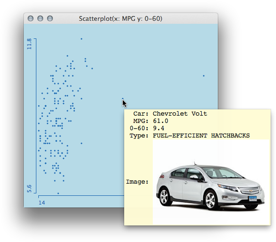
Before discussing the smoothing issues, lets take a look at the dataset. The data can be found at the Consumer Union’s website, and lists basically only 0-60 mph acceleration and fuel efficiency for 168 cars, along of with a classification of the car type. As Mondrian offers the ability to show graphical queries, which pull images directly from the web, I also added a column containing links to images of the cars. Here is an example for the Chevy Volt:

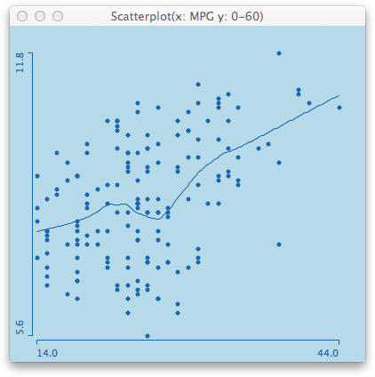
We immediately see two very efficient cars – compared to the rest of the cars – which is the Chevy Volt and the Nissan Leaf. As the examples on the JMP blog leave these two cars out, I chose to do the same. Here is what a smoother for all remaining cars looks like.

Unfortunately, the post on the JMP blog does not tell us which smoother they actually use, but if you compare my result with the first scatterplot in the post, you find quite some differences. Not in the general result, which is better acceleration reduces mileage (what a surprise …), but in the detail interpretation. Whereas the smoother on the JMP blog is quite bumpy, the loess smoother suggest an almost linear relationship except for the range between 20 and 30 mpg, which does not change much even when we change the smoothing parameter.
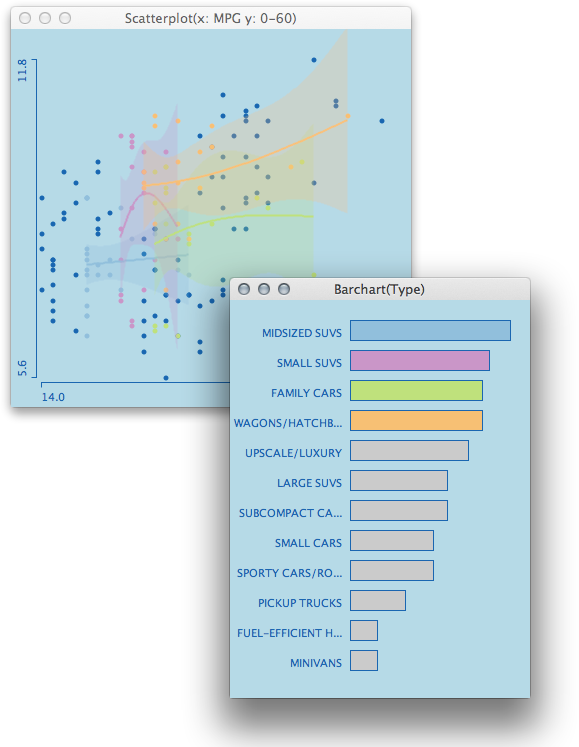
Finding adequate and comparable smoothing parameters is the challenge when showing smoothers for multiple groups (usually of different sizes). For this example, I chose spline smoothers, which also allow to plot a confidence band around the smoothing estimate.
 The example shows natural smoothing splines with 1 df. As the groups differ in size and support along the x-axis, the degree of smoothing looks quite different and somewhat inhomogeneous; which usually should not be the case.
Talking to experts in the field, they only shrugged their shoulders when I asked them, how to find compatible smoothing parameters for different sample sizes.
Btw, the problem was solved on the JMP blog quite elegantly by using linear fits, i.e. no smoothness at all 😉


