Statistical Graphics and more

It’s been too long since the last posting (on barcharts) in the teaching corner. This one will be on histograms.

Histograms are often mistaken with barcharts. The fundamental distinction between the two is

• Barcharts show counts (or weights) for the discrete axis of a categorical variable
• Histograms show an approximation of the density function (if scaled accordingly) of a countinuous variable.

As a consequence, the only thing that can be quantified in a barchart is the bar height (better length, which makes it independent from their orientation). On the other hand, in a histogram, the area of the boxes is proportional to the density approximation. If all bars have the same width in a barcharts, or gaps are drawn in a histogram (which is complete nonsense), the two plots can get mixed up.

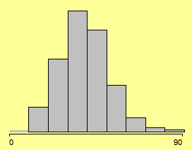
(% votes for Kerry in the 2004 presidential election)

Much has been written about optimal bin width for histograms – almost nothing about the choice of the anchor point. Changing the latter often changes the shape of the histogram more dramatic than choosing between 8, 9 or 10 bins.
Setting the anchor point from 0 to -2.4 yields:

(changing the anchor point to -2.4)

In most applications, there are sensible breaks which can be chosen. Since we look at 3,111 voting districts, we can use far more bins and start at 0 with bin width of 5.

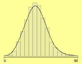
(using meaningful parameters (0, 5) – density estimate added)

If we link a second attribute into the histogram, the whole thing gets more exiting!

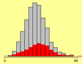
(all districts where more than 15% have a college degree selected)

We don’t really can see what is going on here (although we might guess, that there is a slightly higher proportion of highlighting towards the higher votes for Kerry).

When we use the same normalization trick as for Spineplots (see previous post), we get the clearer picture of the Spinogram:

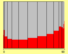
(highlighting in a Spinogram)

Well, that’s what we would have expected, probably except for the increase at the left end of the scale.

The problem with the histograms used so far is that we looked at voting districts, and not at voters! This will distort the impression if the districts are not of equal size. Weighting above histogram will move the mode further to the right.

(the weighted histogram represents voters not districts)

Finally we get the weighted spinogram, which probably supports more the hypothesis … of the selected group.

(the weighted spinogram)

(Sorry for the lengthy post … but concepts get a bit more complex)